Utility Elasticity
Framework
It is typically assumed that utility ($u$) as a function of income ($x$) takes this form: $$ u = \left\{ \begin{array}{ll} \ln{(x)} & \epsilon = 1 \\ \frac{x^{1-\epsilon} - 1}{1 - \epsilon} & \epsilon \gt 0 \end{array} \right. $$ where $ \epsilon $ is non-negative and represents how quickly additional income becomes useless.
Mathy people will note that the $ \epsilon = 1 $ case is the limit of the $ \epsilon \gt 0 $ case.
This formula doesn't have strong justification, but there is a discussion of it here Welfare weights.
Our task is to estimate $\epsilon$.
Common Estimation Methods
- We can assume utility is normally distributed and a function of only income and then solve for $\epsilon$ mathematically. There is no reason to assume utility is normally distributed, and there is plenty of reason to think other things affect it besides income.
- We can assume governments tax everyone such that everyone's utility is decreased equally. Then, we can compute the $\epsilon$ that would imply this is true. There is plenty of reason to doubt that governments either want equal utility cost from their taxes or have the ability to deliver on that goal.
- We can ask people in surveys with hypothetical questions concerning risk and inequality aversion and see what $\epsilon$ there answers are consistent with. There is good evidence that people are horrible at dealing with risk (or numbers more generally). We also have reason to doubt what people say due to the pro-social bias against inequality.
- Evans Evans cites the Binswanger section from Newbery. Unfortunately, I can't find the book.
- We can examine lifetime consumption patterns, which (if people are rational) should be largely determined by $\epsilon$. This assumes people don't hyperbolically discount their future selves, which we know to be false.
- We can use the Fisher-Frisch-Fellner (FFF) model. This is the sole method I think is reasonable, so we'll discuss it more below.
Other Estimation Methods
Some studies use investment returns to estimate risk-aversion. However, your human capital isn't accessible for investment, elasticities measured this way are strongly biased downwards for young investors. Presumably such estimates would be accurate for non-working/older investors, but seeing as many of them buy bonds (a terrible idea) - I'm guessing even in that demographic, we'd generally see results that don't reflect people's true values.
Moreover, the risk-free rate rate of return is literally negative DFII5 right now, so it'd be more accurate to view our financial system as a system for moving risk from risk-intolerant people to risk-tolerant people. For this reason, investment decisions or equilibrium prices (e.g. of options) don't merely reflect the elasticity of utility and income/consumption - they reflect the demographics of the traders weighted by wealth.
Given all of this, I'm skeptical of estimates based on the people's financial decisions or based on financial market equilibrium prices. That being said, there is a plausibility here in that most active money is being invested by hedge funds and wealth tends to be owned by people for whom it is large relative to the net present value of their labor income. From what I've seen, this approach suggests $\epsilon \approx 0$.
Another approach is to infer implied risk-aversion when people choose insurance deductibles and premiums. In addition to traditional irrationality issues, many people are cash/borrowing-constrained in the short-run, which makes short run problems (e.g. car crashes) artificially worse than a naive analysis would entail. Unsurprisingly, such studies find people are absurdly risk averse Cohen. However, given these issues, we'll ignore those.
Finally, one would think that lotteries would provide a way to investigate this, but given that most lotteries are negative-sum, its clear that naive utility maximization is not the major motivation for participating - instead lotteries are more accurately viewed as entertainment row which you buy a ticket.
What follows are what I consider the least-bad methods for estimating human's utility-consumption elasticity.
Subjective Well-Being
We can ask people to rate their well-being on a scale (e.g. from 1-10), assume this is linearly related to utility, and and then find the relationship between consumption and their well-being. This assumes that people's ratings aren't significantly biased by cultural differences.
An analysis of five large surveys controlled for a variety of variables before estimating $\epsilon \approx 1.24$ with standard error 0.05 Layard.
FFF Estimates
The FFF procedure assumes that utility functions are additively separatable between a particular good/service and all other goods and services. This means we can represent utility as $$ u = f(c_0) + g(c_1)$$ where $f$ and $g$ are two utility functions, $c_0$ is how much of some particular good/service is consumed, and $c_1$ is how much of all other goods/services are consumed.
This assumption isn't widely accepted for any good/service. To quote Evans Evans:
Results for $e$ based on the FFF model have generally been disregarded in the literature, mainly on the grounds of the strong condition of additive separability (preference independence) that is required for the approach to be valid.
...
However, in the case of food (and some other broadly defined product groups), Fellner (1967), Selvanathan and Selvanathan (1993) and Evans and Sezer (2002) have all argued that preference independence is a plausible assumption. Furthermore, Selvanathan (1988) tested the want-independence assumption for broad aggregates, using OECD data, and found it to be empirically valid. [However,] both Cowell and Gardiner (1999) and Pearce and Ulph (1999) largely disregard empirical estimates of $e$ based on the model.
In any case, if we accept this is true for some particular good (e.g. food), then we can examine how the demand for food changes when incomes change and when prices change and deduce (with some calculus) what the implied value of $ \epsilon $ is.
Evans then goes on to list some empirical estimates:
| Study | Estimate of $\epsilon$ | Nation |
| Kula (2002) | 1.64 | India |
| Evans and Sezer (2002) | 1.6 | UK |
| Evans (2004a) | 1.25 or 1.6 | UK |
| Evans (2004a) | 1.3 or 1.8 | France |
Groom, et al also attempts to estimate $\epsilon$ with this method and concludes it is 3.6 with standard error 2.2 Groom. Given that enormity of the standard error, I'm inclined to ignore this estimate.
Historical Labor
Suppose, for sake of argument that $\epsilon = 1$. This implies utility is given by $$ u = \ln{(x)} $$
Now suppose labor is additively separatable from consumption and people consume all their income. Now, utility is given by $$ u = \ln{(w \cdot L)} - f(L) $$ where $w$ is the wage and $f$ is some function representing disutility from working.
If we assume people choose $L$ rationally, we can show (with a little calculus) that $$ 1 = L \cdot f'(L) $$
This implies that $L$ is independent of $w$, which means that we should expect people to work the same number of hours regardless of $w$.
Fortunately, we have a natural experiment for this. Over the last couple centuries, the average wage has increased dramatically. $\epsilon = 1$ predicts that labor hasn't changed.
Between 1948 and 2018, real GDP per hour worked increased 3.43-fold while total hours worked increased 2.57-fold Table 1.1.3 Table 1.1.5 Table 6.9B Table 6.9D.
However, during that same time, the US working-age population increased 2.39-fold Working age population, which means we really only saw a 8% increase in labor-per-working-age-person despite a 243% increase in wages.
There have, however, been a number of changes that bias this estimate:
- Women entered the workforce. Their labor force participation increased from 32.7% to 57.1% between 1948 and 2018 Civilian Labor Force Participation Rate: Women. If we naively assume men stayed at their 1948 participation rate of 86.7%, then this represents a 22% increase in laborers per capita. In reality, participation only increased 7% because a significant number of men dropped out Labor Force Participation Rate - Men.
- Transfers and benefits ("welfare") increased between 1948 and 2018 due to a variety of factors such as LBJ's The Great Society, Obamacare, the general rise of health care costs, and the increasing of life expectancy relative to a static retirement age.
- The culture changed in various other ways.
Just to reiterate, despite a 243% increase in wages, hours worked only increased a mere 8% per working-age person. That's remarkably close to the 0% predicted by the $\epsilon = 1$ theory, and, given the uncertainty inherent in #1-3, I think it very fair to conclude the evidence is consistent with the theory.
Now suppose $\epsilon$ was large, say $\epsilon = 2$ (rather than 1), we can model utility as $$ u = -\left(w \cdot L \right)^{-1} - L^\beta $$ where $\beta$ is some constant.
Again, using calculus and assuming rationality, we can prove $$ 1 = w \cdot L^{b+1} $$
Now, suppose this 3.43-fold increase in wages caused $L$ to decrease by 10%. This implies $b = 11.7$, which means shifting the working day from 8 to 9 hours would cause 3.8 times more disutility compared to the change from 7 to 8 hours. This seem ludicrously high to me.
Suppose, instead, $\epsilon = 1.5$ and the same 3.43-fold increase in wages also causes a 10% decrease in $L$. This implies $b = 6.0$, which means shifting the working day from 8 to 9 hours would cause 1.8 times more disutility compared to the change from 7 to 8 hours. This seems more plausible, but still kind of high to me.
This entire section on estimating $\epsilon$ from historical labor trends is rather speculative. However, it suggests to me that $\epsilon$ is probably closer to 1 than 2.
This idea of estimating the elasticity of utility and consumption has been done more rigorously and thoroughly by Raj Chetty Chetty, who ends up also concluding that $\epsilon \approx 1$ and is definitely less than 2.
If we use a binomial distribution to estimate a 95% confidence interval based on his 18 studies in Table 1, we find a range from 0.60 to 1.46, with a center of 1.01.
Overall Estimate
We've estimated $\epsilon$ four different ways:
| Method | $\epsilon$ Estimate |
| Investment Returns | ≈1 |
| Subjective Well-being | 1.15 - 1.33 |
| FFF Procedure | 1.25 - 1.8 |
| Historical Labor | 0.60 - 1.46 |
Britain and France estimate $\epsilon$ as 1 and 2, respectively.
Altogether, it looks likely that $ \epsilon $ is almost certainly less than 2, and probably just above 1. I'd say the balance of the evidence suggests $\epsilon \approx 1.2$.
Public Policy Discount Rates
Using some basic calculus, expected value theory, and an assumption of little change in income inequality, we can prove the discount rate should be $$ p + i + \epsilon \cdot r $$ where $p$ is the probability of social collapse, $i$ is inflation, and $r$ is the expected percent growth in incomes. We're going to ignore $p$ and $i$ and focus on $\epsilon$ and $r$ because
- $p$ is extremely difficult to nail down and also fairly irrelevent for discounting purposes. Even if the probability of humanity going extinct this century is 19% Todd, B., $p$ would be a mere 0.21%.
- $i$ typically doesn't matter unless you own bonds. If inflation is 5% higher, interest rates tend to be 5% higher and the stock market tends to grow 5% faster. In any case, you can compute expected inflation using TIPS spreads 10-Year Breakeven Inflation Rate.
In the US, real GDP per capita growth has averaged 1.6% over the same period, suggesting a discount rate of around 1.9%.
Globally, real GDP per capita has averaged 4.3% growth over the last 28 years GDP per capita, PPP (current international $), which suggests a global discount rate of around 5.2%.
Are things different among the global poor?
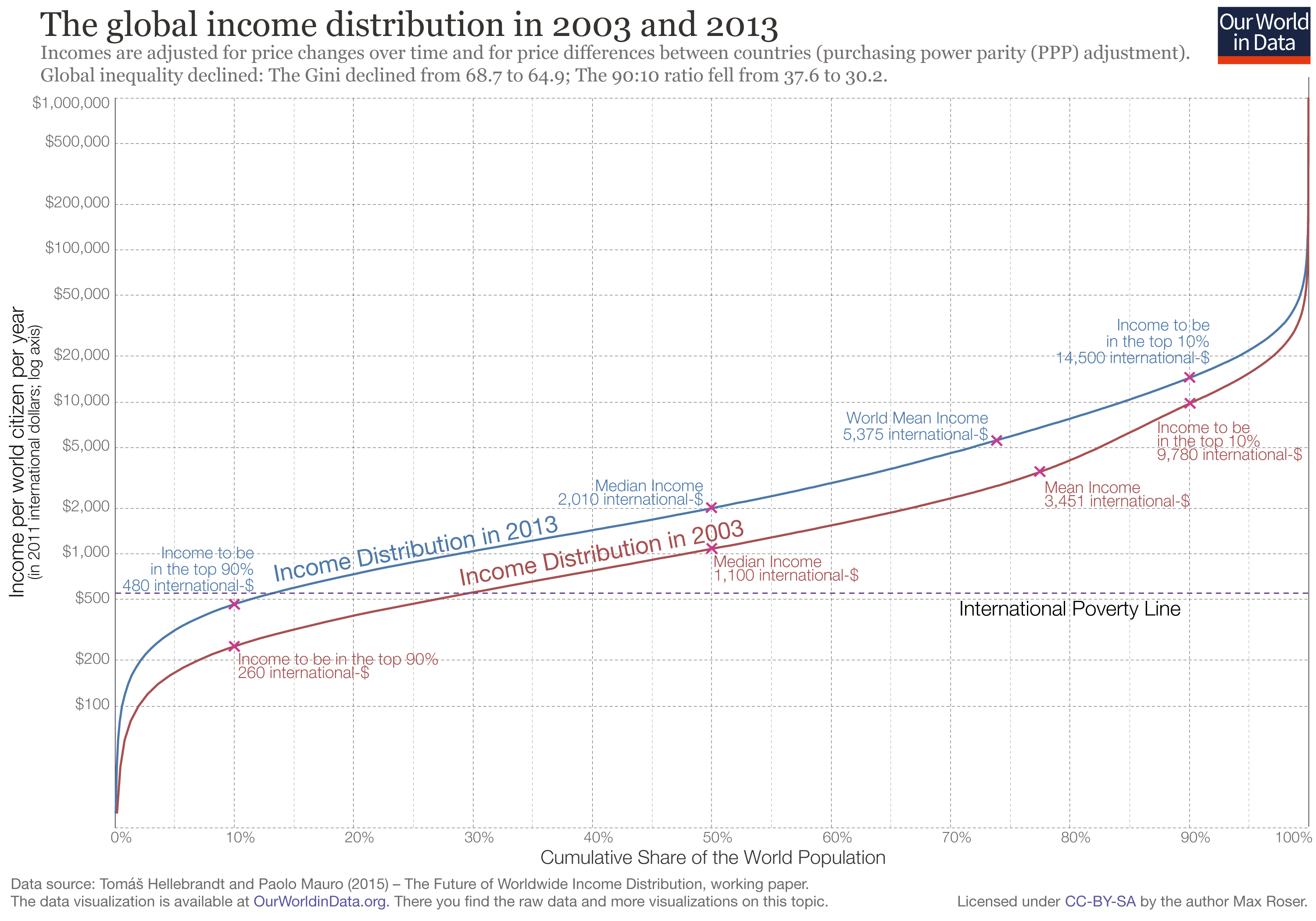
The incomes of people between the 5th percentile and 50th percentile increased by about 6.3% per year between 2003 and 2013. However, real global GDP increased 6.4% over the same time period, indicating that (assuming $\epsilon$ is the same) the discount rate is roughly the same among the global poor as the world at-large (about 5.2%).
Personal Finance Discount Rates
We can combine our estimate of $\epsilon$ with the Markowitz model and historical S&P 500 data to estimate the discount rate people should use when thinking about their finances. Doing so results in a discount rate estimate of just over 7.8% before taxes and 6.0% after taxes.
My Darlings
William Faulkner said good writers need to kill their darlings - to remove the parts of their writing that they personally like a great deal but are ultimately tangential to the story.
But this isn't Faulkner's blog, so, as a compromise, I'm including one of darlings as a link and the other as a couple paragraphs here:
One way to estimate $\epsilon$ is to look at the $\epsilon$ implied by the actions of some of the most rational and numerically literate people on the planet: investors. I've briefly written before on how rational people don't buy bonds but they do buy stocks and housing, the former of which has higher returns and is also higher risk.
It just so happens that the market capitalization of stocks and housing are pretty similar. Referring to my spreadsheet, the expected returns were 8.11% and 5.47% respectively while the covariance matrix of annual returns over 125 years was
| housing | sp500 | |
| housing | 0.0058 | 0.0035 |
| sp500 | 0.0035 | 0.0347 |
Solving for the $\epsilon$ that entails this is rational (via the methodology laid out by me here and also by Markowitz Markowitz) yields an estimate of about 1.8. Moreover, this value is clearly an overestimate because people work and save over decades, which allows them to de-risk relative to the naive just-invest-the-principle model. Indeed, I suspect for reasons laid out here that the true implied $\epsilon$ is much lower. Given the biases inherent in this approach and the degree to which it differs from the other approaches' estimates, I suspect it's not very useful.