Gaussian Processes
Part 1: The Multivariate Gaussian
Gaussian processes are frequently overcomplicated, despite being, at their base, some fairly mundane statistics repackaged in some matrix notation. In the following sequence I'm going to try to break down Gaussian processes.
While beautiful diagrams of a Gaussian Process fit to toy datasets is compelling, an explanation of Gaussian Processes must start, first, with the multivariate normal distribution, as this forms the core of the math that makes a Gaussian Process work.
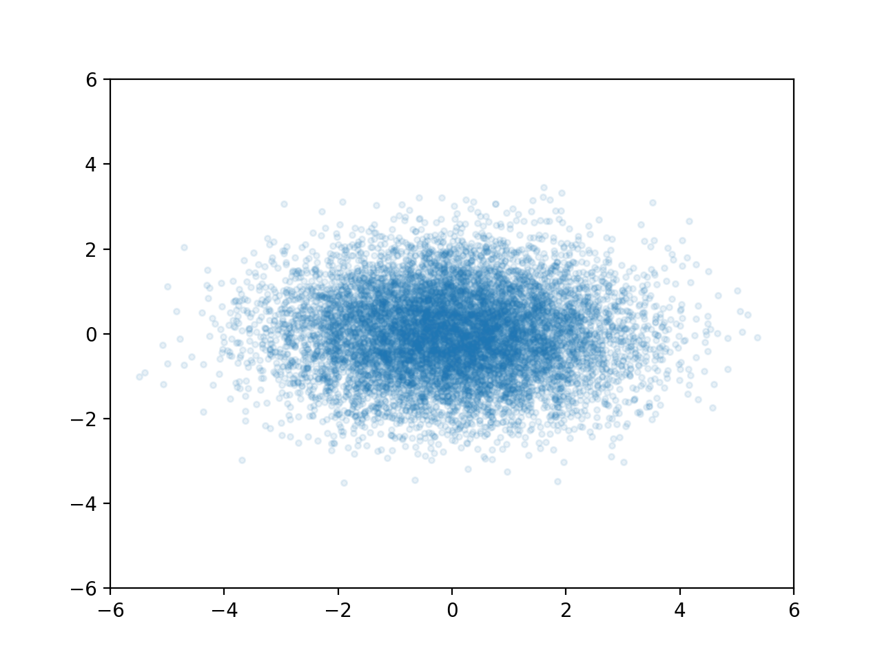
Consider the point cloud below. It is an example of a 2D Gaussian distribution.
The two dimensions are independent which means that knowing a randomly selected point's X value doesn't tell us anything about its Y value (and vice versa).
A multivariate Gaussian distribution is any linear transformation of independent Gaussian variables. For instance if we use $X_2 = X_1$ and $Y_2 = X_1 + Y_1$ we can transform the cloud above into this.
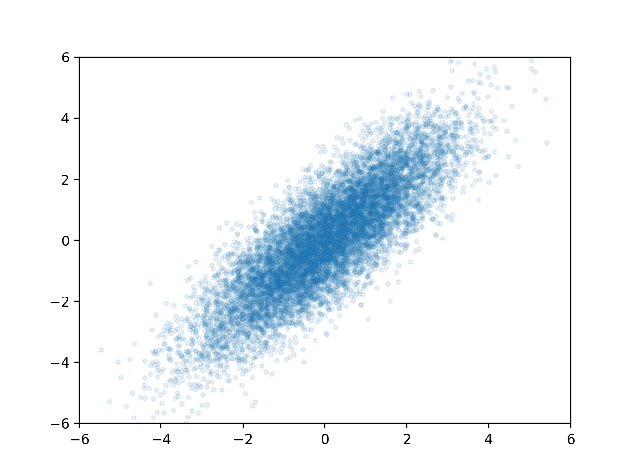
This one is much more interesting. Now the X and Y values of points are linearly correlated, which means if I know the X value of a randomly selected point, it gives me some information about it's Y value. For instance, if I know the point's X-value is around 2, then I know its Y-value is around 2 as well. In fact, let's take a look at the Y-values where X is close to 2:
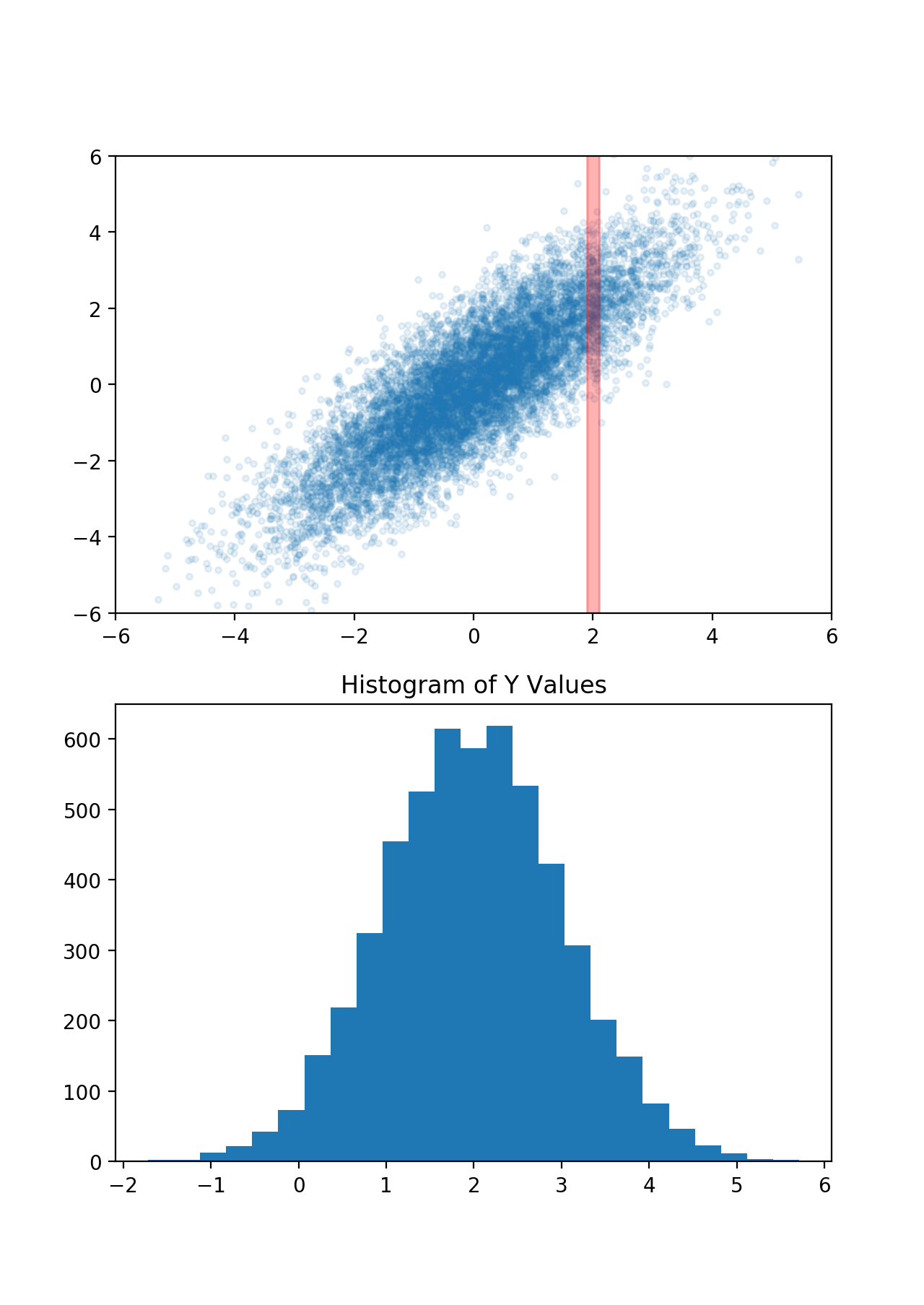
This is, in fact, another Gaussian distribution, which has a mean of 2 and a variance of 1. In other words, since we know one thing about our point (its X-value), our best prediction for another thing (its Y-value) changed, and our uncertainty was reduced.
This forms the core of what a Gaussian Process does: you tell it how correlated some different variables are, as well as some variables that you already know, and the Gaussian Process tells you the corresponding prediction for values you don't know.
Your prediction for the Y-value before you know anything is called your prior — in this case it was a Gaussian with mean = 0 and variance = 2.5. Your prediction after you "condition on" some information is called your posterior — in this case a Gaussian with a mean of 2 and a variance of 1.
Math
WARNING: Copious amounts of matrices beyond this point
The idea above of taking a "slice" of a prior to get a posterior can be applied to any distribution, but is particularly elegant for the Gaussian distribution, since the math tends to be (relatively) efficient and the result is always another Gaussian distribution.
The typical representation of a D-dimensional multivariate Gaussian distribution is to have a vector that stores the center of the distribution called \(\mu\) and a DxD covariance matrix called \(\Sigma\): \[ p(X=\vec{x}) = \mathcal{N}(\vec{\mu}, \Sigma) \] $\Sigma_{ij}$ is the covariance between dimensions $i$ and $j$. $\Sigma_{ii}$ is the variance of dimension i.
As an example, suppose you have the following 2-dimension Gaussian distribution: \[ p(X = x, Y = y) = \mathcal{N}([\mu_x, \mu_y], \begin{bmatrix} \sigma_x^2 & \text{cov}(x, y)\\ \text{cov}(x, y) & \sigma_y^2 \end{bmatrix} )\] If we know the x coordinate of a particular point, this gives us new information about what its y value might be. As we saw above, our updated guess for y is a Gaussian distribution, but we didn't see the actual math for computing the mean and variance of that distribution. The formulae are: \[\mu_{y (new)} = \mu_{y (old)} + \frac{\Sigma_{x,y}}{\Sigma_{y,y}} (x - \mu_x)\] \[ \sigma_{y (new)} = \sigma_{y (old)}^2 - \frac{\Sigma_{x,y}^2}{\Sigma_{x,x}} \]
The more standard nomenclature is to say that the "new" distribution (the posterior) is "conditioned" on our knowledge of x. In this case "|" is the mathematical symbol for "conditioned on", so we can re-write the above equations:
\[\mu_{y|x} = \mu_{y} + \frac{\Sigma_{x,y}}{\Sigma_{y,y}} (x - \mu_x)\] \[ \Sigma_{y|x} = \sigma_{y}^2 - \frac{\Sigma_{x,y}^2}{\Sigma_{x,x}} \]Unfortunately, the equations for more than two dimensions are quite complicated, but (fortunately) they can be expressed in matrix notation quite nicely. Suppose you know the first $N$ dimensions of a sample from a $D$ dimensional multivariate Gaussian distribution, and would like to know your posterior on the remaining dimensions. Then we can organize $\Sigma$ into four corners:
\[ \Sigma = \begin{bmatrix} \Sigma_{11} & \Sigma_{12}\\ \Sigma_{21} & \Sigma_{22} \end{bmatrix} \]Here $\Sigma_{11}$ is the covariance matrix of the first $N$ dimensions and $\Sigma_{22}$ is the covariance matrix of the remaining dimensions. $\Sigma_{12}$ and $\Sigma_{21}$ are the covariances between the dimensions you know and the dimensions you don't know (note that \(\Sigma_{12} = \Sigma_{21}^T\)). Then your posterior is a normal distribution with the following mean and covariance matrices:
Conclusion
What does any of this have to do with Gaussian Processes? Well the steps you take when using a Gaussian Process are
- Tell the Gaussian Process your initial guess for the means of each dimension
- Tell the Gaussian Process the covariance between each dimension
- Apply the formula above
That's it! Gaussian Processes are just the Machine Learning community's take on the multivariate Gaussian distribution, using machinery that has been known for more than a century. They're wrapped in different terminology and have some tricks that would turn a statistician's stomach, but at it's core it's just conditioning (i.e. "taking slices of") Gaussian distributions.
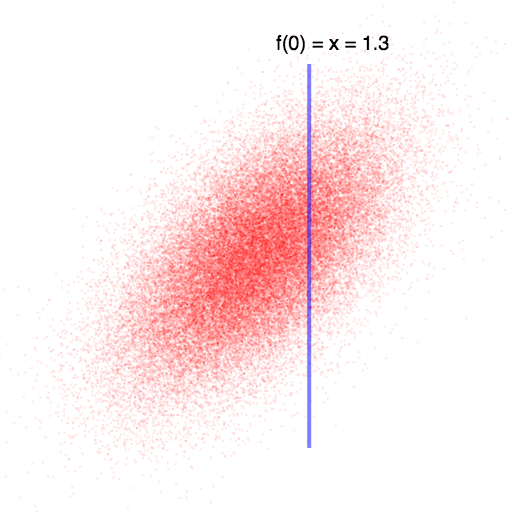
In this case, knowing that $f(0)$ is higher than we expected leads us to believe that $f(1)$ will also be higher than we expected (since they are positively correlated). Once we observe f(0), we can compute the exact values for f(1) using the Gaussian-conditioning formula above.
Unfortunately, many real world problems have uncountably many possible inputs. A far more common case is trying to learn a function that maps real numbers to real numbers: \[ f: \mathbb{R} \rightarrow \mathbb{R} \] A Gaussian Process will reason about this the exact same way it reasoned about the discrete case: it will form a Gaussian distribution such that every possible input-value has a corresponding pdf over its possible output values. Then it will look at the values/dimensions that it does know (i.e. the "training set" or "observations") and use this knowledge to compute a new multivariate distribution over all dimensions that it wants to predict.
At first blush, it seems rather dubious that the machinery we used for finite-dimensional multivariate Gaussian distributions would work well (computationally) for infinite-dimensional Gaussian distributions. In fact, such skepticism would be well placed! Recall the definition from the beginning of the article:
Def: A Gaussian Process is a collection of random variables, any finite number of which have a joint Gaussian distribution
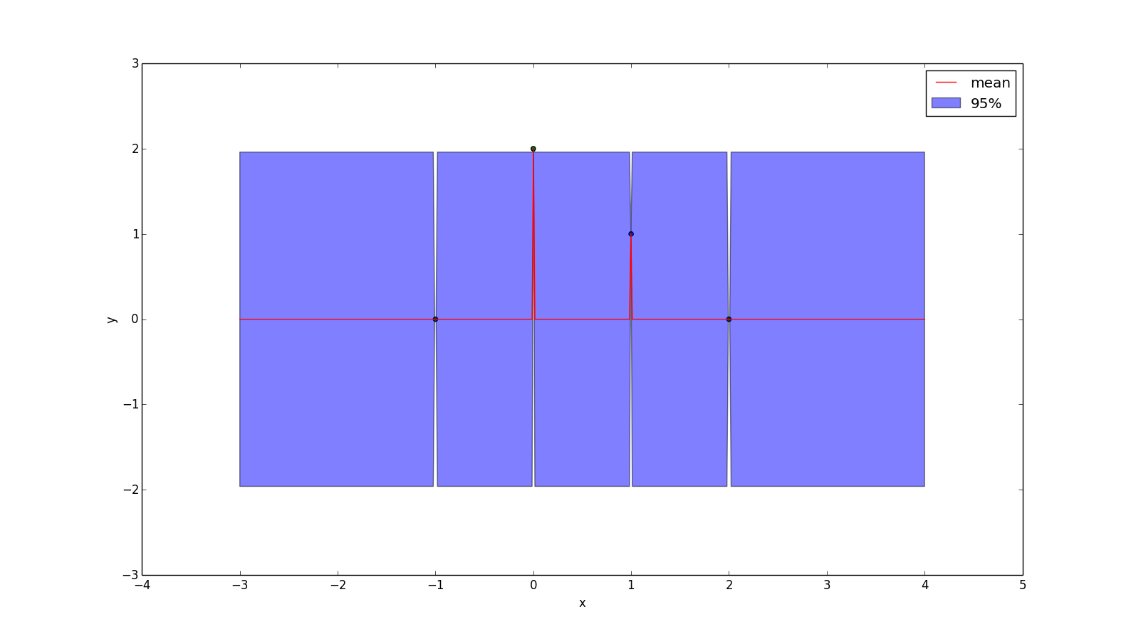
The key is that we only ever care about the Gaussian distribution at a finite number of points. For example, consider this case:
 We only know the input at 4 locations, and so if we want to determine our prediction of the function at some other point (e.g. x = 0.5), we just form a 5-dimensional multivariate Gaussian distribution, condition on the dimensions we know and see what the resulting distribution is for the dimension we want to know. So if I want to know my posterior at $x = \frac{1}{2}$, then I'm just computing
\[ p(f(\frac{1}{2})\ |\ f(-1), f(0), f(1), f(2))\]
We only know the input at 4 locations, and so if we want to determine our prediction of the function at some other point (e.g. x = 0.5), we just form a 5-dimensional multivariate Gaussian distribution, condition on the dimensions we know and see what the resulting distribution is for the dimension we want to know. So if I want to know my posterior at $x = \frac{1}{2}$, then I'm just computing
\[ p(f(\frac{1}{2})\ |\ f(-1), f(0), f(1), f(2))\]
If $k(x_1, x_2)$ is a function that returns the covariance of $f(x_1)$ and $f(x_2)$, then we can write \(Sigma\) as \[ \Sigma = \begin{bmatrix} k(-1, -1) & k(-1, 0) & k(-1, 1) & k(-1, 2) & k(-1, \frac{1}{2})\\ k(0, -1) & k(0, 0) & k(0, 1) & k(0, 2) & k(0, \frac{1}{2})\\ k(1, -1) & k(1, 0) & k(1, 1) & k(1, 2) & k(1, \frac{1}{2})\\ k(2, -1) & k(2, 0) & k(2, 1) & k(2, 2) & k(2, \frac{1}{2})\\ k(\frac{1}{2}, -1) & k(\frac{1}{2}, 0) & k(\frac{1}{2}, 1) & k(\frac{1}{2}, 2) & k(\frac{1}{2}, \frac{1}{2}) \end{bmatrix} \] In the above example, I assume $\mu = 0$ (i.e. my prior is that the points are normally distributed around f(x) = 0), then this gives us all we need to plug-and-chug with the Gaussian-conditioning formula: \[ p(\vec{x}_2 | \vec{x}_1) = \mathcal{N}(\vec{\mu}_{2|1}, \Sigma_{22|1})\] \[\vec{\mu}_{2|1} = \vec{\mu}_2 + \Sigma_{21} \Sigma_{11}^{-1} (X_1 - \vec{\mu}_1)\] \[\Sigma_{22|1} = \Sigma_{22} - \Sigma_{21} \Sigma_{11}^{-1} \Sigma_{12}\] The y-value of the red line at $x = \frac{1}{2}$ in the image above is simply the mean of the normal distribution that results from conditioning on the four points that were observed. The 95% range is calculated from the variance of the resulting normal distribution.
Noise
As you may have noticed, I have been assuming our observations of the function are perfect, but in practice it is often useful to assume normally distributed noise. Adding noise is a simple matter of adding $\sigma^2 I$ to $k(X,X)$: \[ p(y_* | \vec{X}_*, X, \vec{y}) = \mathcal{N}(\vec{\mu}, \Sigma)\] \[\mu = k(X_*, X) (k(X,X) + \sigma^2 I)^{-1} y\] \[\Sigma = k(X_*, X_*) - k(x_*, X) (k(X,X) + \sigma^2 I)^{-1} k(X, X_*)\]
If we add noise with a mean of zero and a standard deviation of 0.1, then the example we've been using becomes:
Food for thought: why is adding $\sigma^2 I$ to the covariance matrix the correct way to model iid Gaussian noise?

Note that we now have some degree of uncertainty everywhere — even at the points we have observed. What is harder to see is that the mean-line (red) doesn't even pass through our observations anymore, as it tends more towards our prior (y=0).
Non-zero Prior
The mean line in the above images tends towards zero when it lacks any other information. While this may be reasonable in some situations, in other cases it can be appropriate to have your "uninformed prediction" (i.e. your "prior") be something else.
Let $\bar{y}(X)$ yield your prior guess for every point in $X$. Then:
\[ p(y_* | \vec{X}_*, X, \vec{y}) = \mathcal{N}(\vec{\mu}, \Sigma)\]
\[\mu = \bar{y}(X_*) + k(X_*, X) (K + \sigma^2 I)^{-1} (y - \bar{y}(X))\]
\[\Sigma = k(X_*, X_*) - k(x_*, X) (K + \sigma^2 I)^{-1} k(X, X_*)\]
The effect of applying the prior $\bar{y}(x) = x$ to the example above is shown below. One interesting thing to note is that, while the mean prediction at every point is different, the uncertainty around the mean is no different than before, because the formula for conditional variance is not affected by our prior.
Kernels
So far we have simply assumed the existence of some function $k(x_1, x_2)$, that returns the covariance of $f(x_1)$ and $f(x_2)$. In other words: \[ \Sigma = \begin{bmatrix} \text{k}(X_1, X_1) & \dots & \text{k}(X_1, X_n)\\ \vdots & \ddots & \vdots\\ \text{k}(X_n, X_1) & \dots & \text{k}(X_n, X_n)\\ \end{bmatrix}\] The fact that covariance matrices are positive semidefinite imposes some restrictions on what this function can be.
Mercer's Theorem:
$k(X, X)$ is positive semidefinite for any collection of points $X = \begin{bmatrix} x_1, \dots, x_n \end{bmatrix}$
if and only iff
$k(x_1, x_2)$ is symmetric (i.e. $k(x_1, x_2) = k(x_2, x_1)$) and can be expressed as an inner product of some feature expansion: \[ k(x_1, x_2) = \langle \phi(x_1), \phi(x_2) \rangle \]
This theorem leads to an interesting interpretation of Gaussian Processes, which is that any kernel function you pick is implicitly a choice of a feature expansion. In fact Gaussian Processes can alternatively be derived by rewriting (Bayesian) linear regression in a kernelized form (proof).
More About Kernels
A kernel $k(x_1, x_2)$ is stationary if it can be written as a function of the difference between $x_1$ and $x_2$.
Let $k_1$ and $k_2$ be kernels and let $c > 0$. Then the following are also kernels: \[ k_3(x_1, x_2) = k_1(x_1, x_2) + c\] \[ k_3(x_1, x_2) = k_1(x_1, x_2) \cdot c\] \[ k_3(x_1, x_2) = k_1(x_1, x_2) + k_2(x_1, x_2)\] \[ k_3(x_1, x_2) = k_1(x_1, x_2) \cdot k_2(x_1, x_2)\]
Examples of Kernels
-
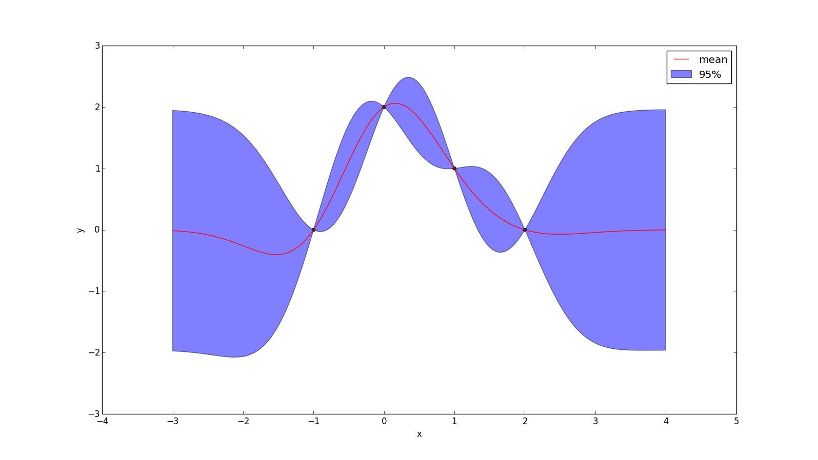
One of the most popular kernels is called the Gaussian Kernel, Squared Exponential Kernel, or Radial Basis Function
\[ k(x_1, x_2) = 2\sigma^2 e^{\frac{(x_1 - x_2)^2}{-2l^2}} \]
Which has two hyper parameters: $\sigma$ and $l$. This kernel can be viewed as only considering functions that are infinitely differentiable (in other words, the mean function will always be nice and smooth). An example is given below, with $\sigma = l = 1$.
-
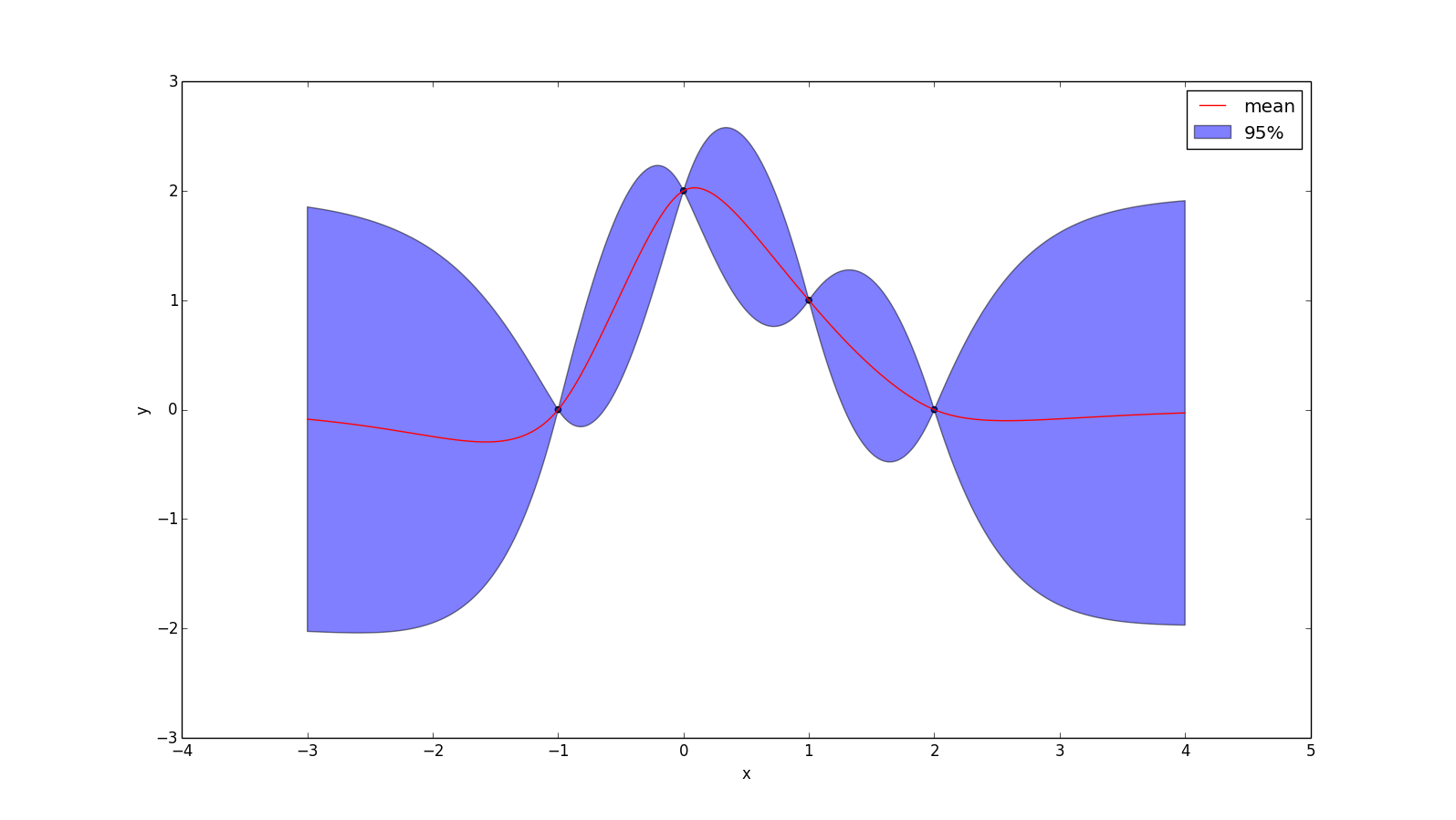
But some would say it is too smooth for practical use! The Matérn kernel weakens these requirements a bit. Technically the Matérn kernel is a very wide class of kernels specified by a hyperparameter v. The most popular ones have $v = 1.5$ and $v = 2.5$, which can be written as
\[k_{v=1.5}(r) = (1 + \frac{r\sqrt{3}}{l}) \cdot \text{exp}(\frac{r \sqrt{3}}{-l})\]
\[k_{v=2.5}(r) = (1 + \frac{r\sqrt{5}}{l} + \frac{5r^2}{3l^2}) \cdot \text{exp}(\frac{r \sqrt{5}}{-l})\]
Where $r = |x_1 - x_2|$. These represent forming a prior over functions that are once and twice differentiable (respectively). Choosing $v > 2.5$ tends to make functions "too smooth" for real problems, while $v < 1.5$ is too rough. An example with $v = 1.5$ and $l = 1.0$ is given below:
-
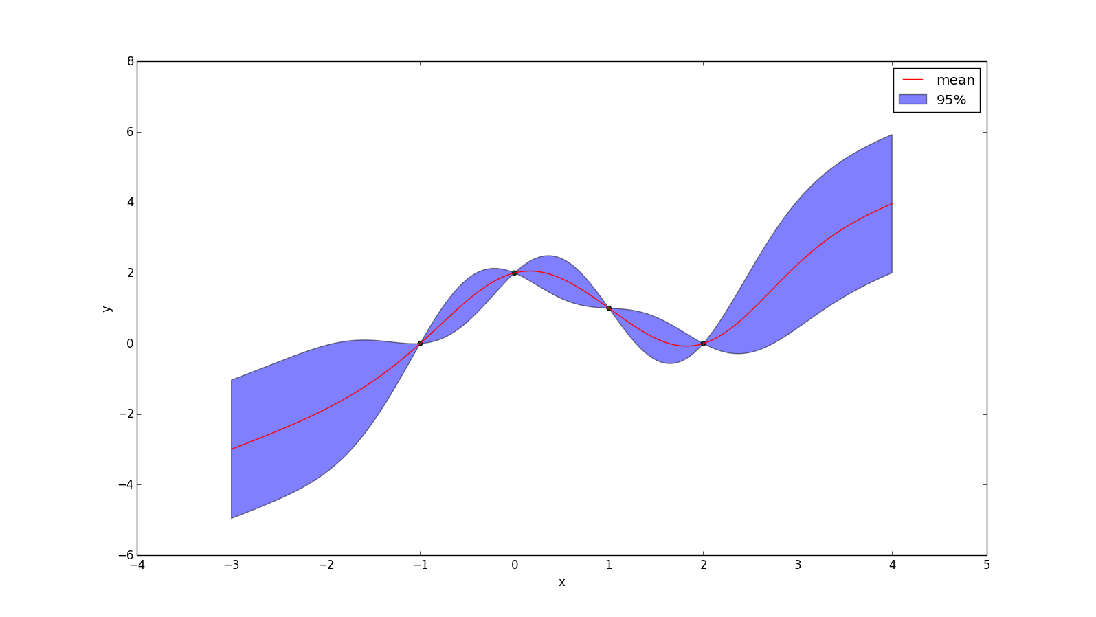
Another useful kernel is the polynomial kernel, which is the kernel-representation of the feature expansion
\[ \phi(x) = [1, x, x^2, x^3, x^4, ..., x^p] \]
The corresponding kernel is:
\[ k(x_1, x_2) = (x_1^T x_2 + 1)^p \]
When $p=1$ the resulting mean function will be the least-squares regression line. When $p=2$ it will be the least-squares quadratic curve. The plot below uses $p=2$ and a noise with standard deviation 0.1.
(Food for thought: if I don't add noise to this, the plotting program crashes. Why do you think that is?)
-
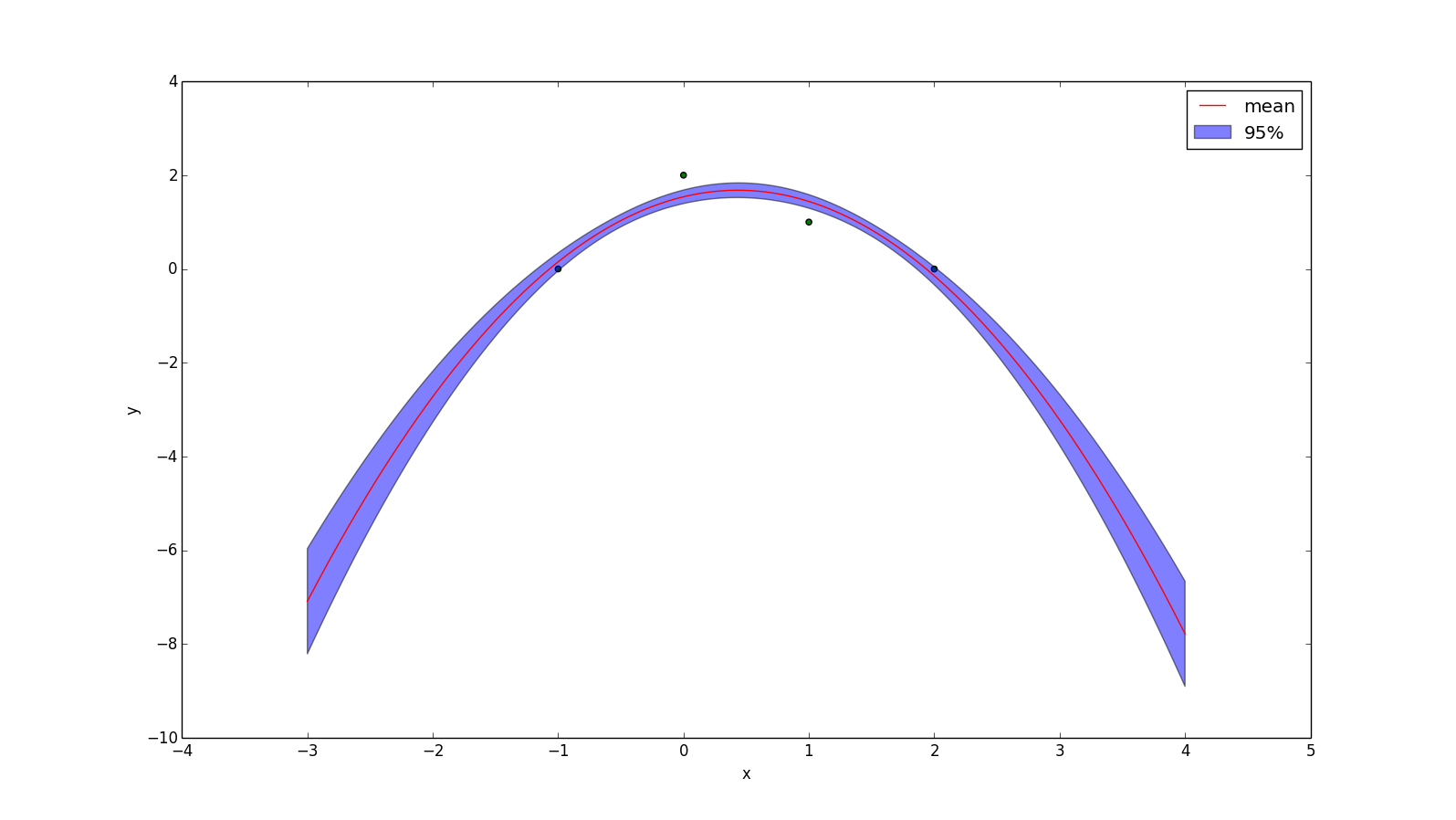
An unpopular kernel is the Dirac delta function:
\[k(x_1, x_2) = \delta(x_1 - x_2)\]
But for didatic purposes, here is the plot:
 This kernel assumes there is no relationship between points!