Gaussian Processes 2: The Kernel Trick
We'll take a bit of a detour now to remark on the connection between Gaussian Processes and linear regression. If (X, Y) are our training set, and are N-by-D and N-by-1 matrices respectively, and Z is our test set, then our predicted labels for Z is given by:
$$Z (X^T X)^{-1} X^T Y$$With a short proof we can prove this is equivalent to:
$$= Z X^T (XX^T)^{-1} Y$$(an astute reader will note that $X X^T$ and $X^T X$ cannot both be invertible if X is not square. We can fix this by adding a tiny amount of regularization, but that distracts from the point...)
This re-write is called Kernel Linear Regression. It is actually strikingly similar to our formula for a Gaussian Process's mean line:
$$ \vec{\mu}_{2|1} = \Sigma_{21} \Sigma_{11}^{-1} X_1 $$Recall that $X_1$ are the points we know the true values of, $\Sigma_{11}$ is how similar the points we know are to each other, and $\Sigma_{21}$ is how similar the points we know are to the points we don't know.
If $\Sigma_{21} = Z^T X$ and $\Sigma_{22} = X^T X$, then this is a perfect fit! In other words, the mean line of a Gaussian Process corresponds exactly to Kernel Linear Regression.
</Detour>
A Gaussian Process assigns every possible input-value a "dimension" in a multivariate Gaussian distribution. For example, suppose you have a function you are trying to "learn" that takes in either a 0 or a 1 and spits out a real number: \[ f: \{0, 1\} \rightarrow \mathbb{R} \] Then in the image below, we could let the "x-axis" represent our belief over the value of $f(0)$ and the "y-axis" represent our belief over the value of $f(1)$. If we know the value of $f(0)$ (by observing it), then this may give us some information about the value of $f(1)$.
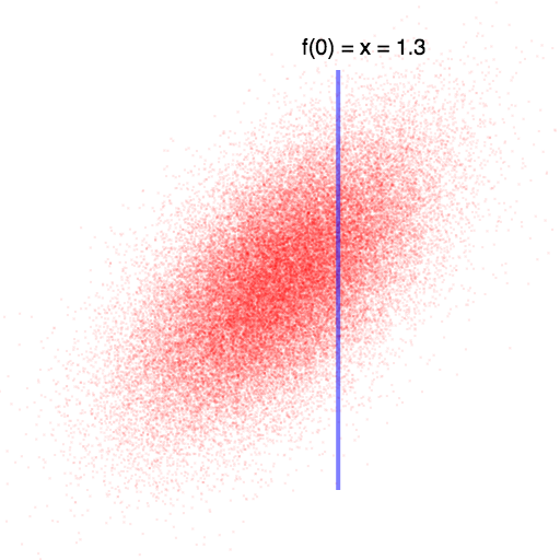
In this case, knowing that $f(0)$ is higher than we expected leads us to believe that $f(1)$ will also be higher than we expected (since they are positively correlated). Once we observe f(0), we can compute the exact values for f(1) using the Gaussian-conditioning formula above.
Unfortunately, many real world problems have uncountably many possible inputs. A far more common case is trying to learn a function that maps real numbers to real numbers: \[ f: \mathbb{R} \rightarrow \mathbb{R} \] A Gaussian Process will reason about this the exact same way it reasoned about the discrete case: it will form a Gaussian distribution such that every possible input-value has a corresponding pdf over its possible output values. Then it will look at the values/dimensions that it does know (i.e. the "training set" or "observations") and use this knowledge to compute a new multivariate distribution over all dimensions that it wants to predict.
At first blush, it seems rather dubious that the machinery we used for finite-dimensional multivariate Gaussian distributions would work well (computationally) for infinite-dimensional Gaussian distributions. In fact, such skepticism would be well placed! Recall the definition from the beginning of the article:
Def: A Gaussian Process is a collection of random variables, any finite number of which have a joint Gaussian distribution
The key is that we only ever care about the Gaussian distribution at a finite number of points. For example, consider this case:
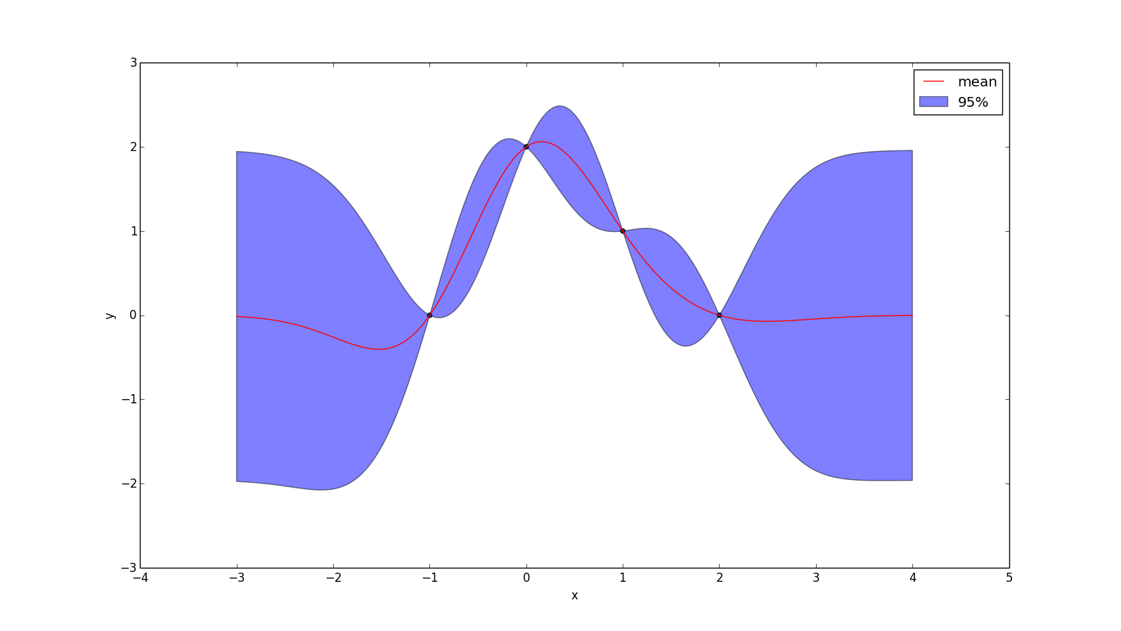 We only know the input at 4 locations, and so if we want to determine our prediction of the function at some other point (e.g. x = 0.5), we just form a 5-dimensional multivariate Gaussian distribution, condition on the dimensions we know and see what the resulting distribution is for the dimension we want to know. So if I want to know my posterior at $x = \frac{1}{2}$, then I'm just computing
\[ p(f(\frac{1}{2})\ |\ f(-1), f(0), f(1), f(2))\]
We only know the input at 4 locations, and so if we want to determine our prediction of the function at some other point (e.g. x = 0.5), we just form a 5-dimensional multivariate Gaussian distribution, condition on the dimensions we know and see what the resulting distribution is for the dimension we want to know. So if I want to know my posterior at $x = \frac{1}{2}$, then I'm just computing
\[ p(f(\frac{1}{2})\ |\ f(-1), f(0), f(1), f(2))\]
If $k(x_1, x_2)$ is a function that returns the covariance of $f(x_1)$ and $f(x_2)$, then we can write $\Sigma$ as \[ \Sigma = \begin{bmatrix} k(-1, -1) & k(-1, 0) & k(-1, 1) & k(-1, 2) & k(-1, \frac{1}{2})\\ k(0, -1) & k(0, 0) & k(0, 1) & k(0, 2) & k(0, \frac{1}{2})\\ k(1, -1) & k(1, 0) & k(1, 1) & k(1, 2) & k(1, \frac{1}{2})\\ k(2, -1) & k(2, 0) & k(2, 1) & k(2, 2) & k(2, \frac{1}{2})\\ k(\frac{1}{2}, -1) & k(\frac{1}{2}, 0) & k(\frac{1}{2}, 1) & k(\frac{1}{2}, 2) & k(\frac{1}{2}, \frac{1}{2}) \end{bmatrix} \] In the above example, I assume $\mu = 0$ (i.e. my prior is that the points are normally distributed around f(x) = 0), then this gives us all we need to plug-and-chug with the Gaussian-conditioning formula: \[ p(\vec{x}_2 | \vec{x}_1) = \mathcal{N}(\vec{\mu}_{2|1}, \Sigma_{22|1})\] \[\vec{\mu}_{2|1} = \vec{\mu}_2 + \Sigma_{21} \Sigma_{11}^{-1} (X_1 - \vec{\mu}_1)\] \[\Sigma_{22|1} = \Sigma_{22} - \Sigma_{21} \Sigma_{11}^{-1} \Sigma_{12}\] The y-value of the red line at $x = \frac{1}{2}$ in the image above is simply the mean of the normal distribution that results from conditioning on the four points that were observed. The 95% range is calculated from the variance of the resulting normal distribution. For visualizations we can just take the main diagonal of $\Sigma_{22|1}$ as the variance at each point.
Noise
As you may have noticed, I have been assuming our observations of the function are perfect, but in practice it is often useful to assume normally distributed noise. This can be accomplished by adding the identity matrix scaled by the noise's variance to \Sigma_{21}. Our updated formulas are: \[\vec{\mu}_{2|1} = \vec{\mu}_2 + \Sigma_{21} (\Sigma_{11} + I\sigma^2)^{-1} (X_1 - \vec{\mu}_1)\] \[\Sigma_{22|1} = \Sigma_{22} - \Sigma_{21} (\Sigma_{11} + I\sigma^2)^{-1} \Sigma_{12}\]
If we add noise with a mean of zero and a standard deviation of 0.1, then the example we've been using becomes:
Food for thought: why is adding $I \sigma^2$ to the covariance matrix the correct way to model iid Gaussian noise?
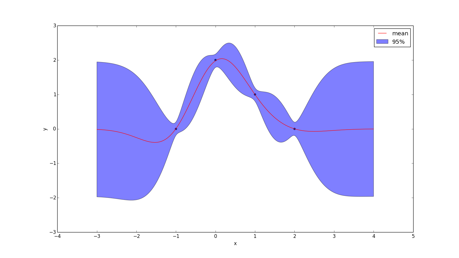
Note that we now have some degree of uncertainty everywhere — even at the points we have observed. What is harder to see is that the mean-line (red) doesn't even pass through our observations anymore, as it tends more towards our prior (y=0).
Non-zero Prior
The mean line in the above images tends towards zero when it lacks any other information. While this may be reasonable in some situations, in other cases it can be appropriate to have your "uninformed prediction" (i.e. your "prior") be something else.
Let $\bar{y}(X)$ yield your prior guess for every point in $X$. Then:
\[ p(y_* | \vec{X}_*, X, \vec{y}) = \mathcal{N}(\vec{\mu}, \Sigma)\]
\[\mu = \bar{y}(X_*) + k(X_*, X) (K + \sigma^2 I)^{-1} (y - \bar{y}(X))\]
\[\Sigma = k(X_*, X_*) - k(x_*, X) (K + \sigma^2 I)^{-1} k(X, X_*)\]
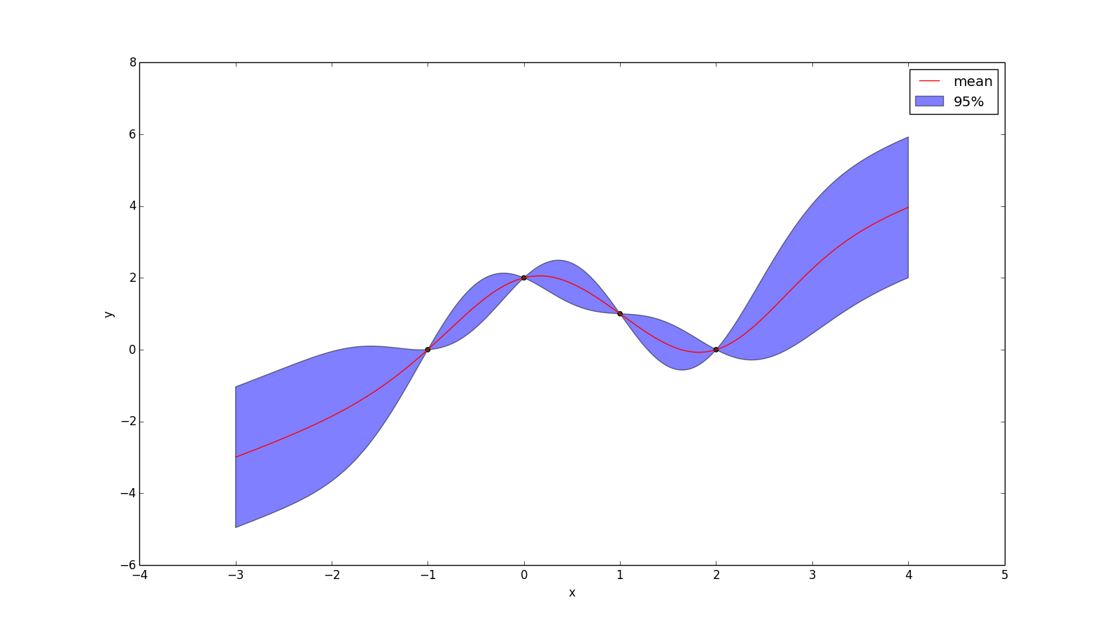
The effect of applying the prior $\bar{y}(x) = x$ to the example above is shown below. One interesting thing to note is that, while the mean prediction at every point is different, the uncertainty around the mean is no different than before, because the formula for conditional variance is not affected by our prior.
Kernels
So far we have simply assumed the existence of some function $k(x_1, x_2)$, that returns the covariance of $f(x_1)$ and $f(x_2)$. In other words: \[ \Sigma = \begin{bmatrix} \text{k}(X_1, X_1) & \dots & \text{k}(X_1, X_n)\\ \vdots & \ddots & \vdots\\ \text{k}(X_n, X_1) & \dots & \text{k}(X_n, X_n)\\ \end{bmatrix}\] The fact that covariance matrices are positive semidefinite imposes some restrictions on what this function can be.
Mercer's Theorem:
$k(X, X)$ is positive semidefinite for any collection of points $X = \begin{bmatrix} x_1, \dots, x_n \end{bmatrix}$
if and only iff
$k(x_1, x_2)$ is symmetric (i.e. $k(x_1, x_2) = k(x_2, x_1)$) and can be expressed as an inner product of some feature expansion: \[ k(x_1, x_2) = \langle \phi(x_1), \phi(x_2) \rangle \]
This theorem leads to an interesting interpretation of Gaussian Processes, which is that any kernel function you pick is implicitly a choice of a feature expansion. In fact Gaussian Processes can alternatively be derived by rewriting (Bayesian) linear regression in a kernelized form (proof).
More About Kernels
A kernel $k(x_1, x_2)$ is stationary if it can be written as a function of the difference between $x_1$ and $x_2$.
Let $k_1$ and $k_2$ be kernels and let $c > 0$. Then the following are also kernels: \[ k_3(x_1, x_2) = k_1(x_1, x_2) + c\] \[ k_3(x_1, x_2) = k_1(x_1, x_2) \cdot c\] \[ k_3(x_1, x_2) = k_1(x_1, x_2) + k_2(x_1, x_2)\] \[ k_3(x_1, x_2) = k_1(x_1, x_2) \cdot k_2(x_1, x_2)\]
Examples of Kernels
-
One of the most popular kernels is called the Gaussian Kernel, Squared Exponential Kernel, or Radial Basis Function
\[ k(x_1, x_2) = 2\sigma^2 e^{\frac{(x_1 - x_2)^2}{-2l^2}} \]
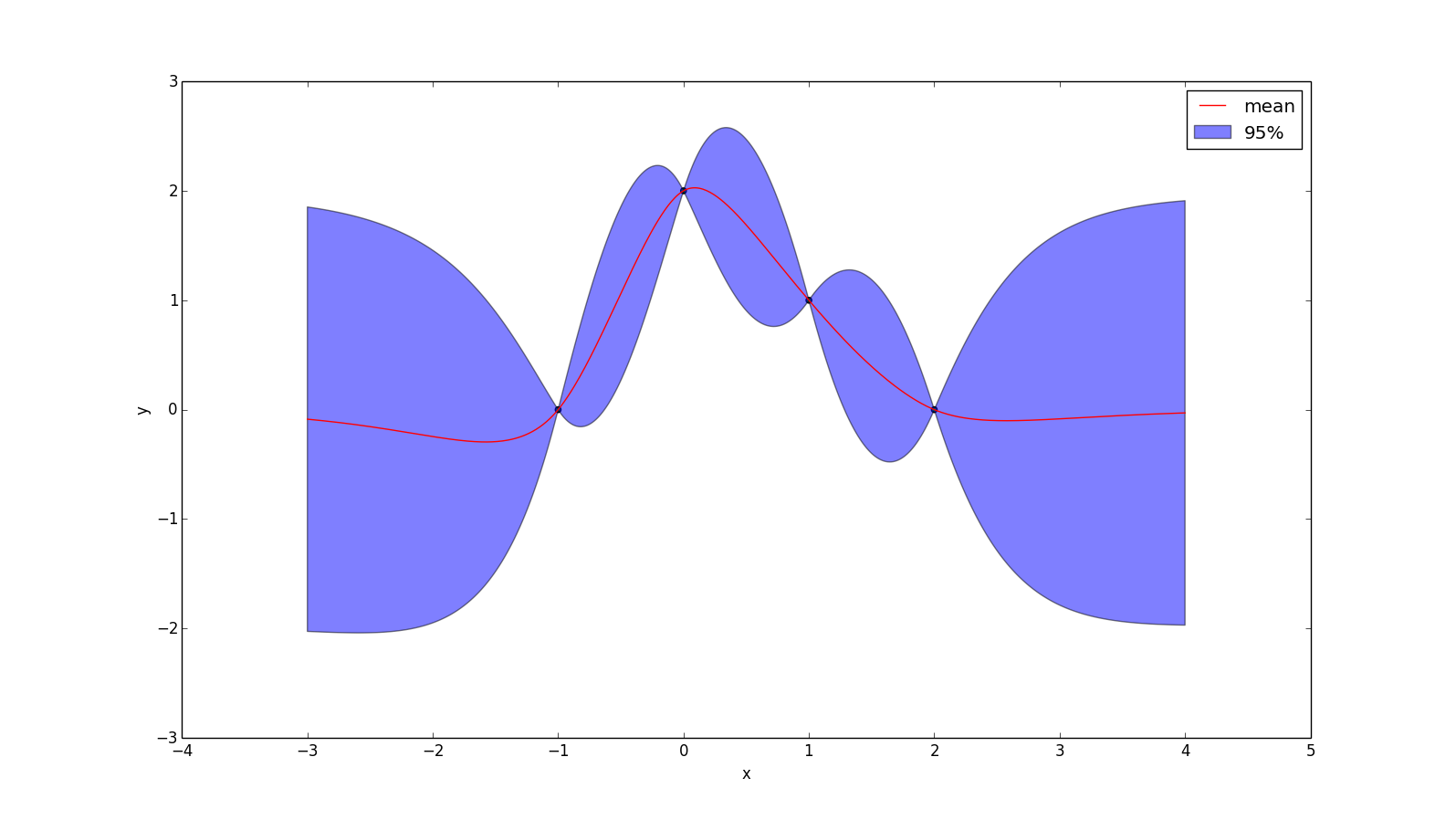
Which has two hyper parameters: $\sigma$ and $l$. This kernel can be viewed as only considering functions that are infinitely differentiable (in other words, the mean function will always be nice and smooth). An example is given below, with $\sigma = l = 1$.
-
But some would say it is too smooth for practical use! The Matérn kernel weakens these requirements a bit. Technically the Matérn kernel is a very wide class of kernels specified by a hyperparameter v. The most popular ones have $v = 1.5$ and $v = 2.5$, which can be written as
\[k_{v=1.5}(r) = (1 + \frac{r\sqrt{3}}{l}) \cdot \text{exp}(\frac{r \sqrt{3}}{-l})\]
\[k_{v=2.5}(r) = (1 + \frac{r\sqrt{5}}{l} + \frac{5r^2}{3l^2}) \cdot \text{exp}(\frac{r \sqrt{5}}{-l})\]
Where $r = |x_1 - x_2|$. These represent forming a prior over functions that are once and twice differentiable (respectively). Choosing $v > 2.5$ tends to make functions "too smooth" for real problems, while $v < 1.5$ is too rough. An example with $v = 1.5$ and $l = 1.0$ is given below:
-
Another useful kernel is the polynomial kernel, which is the kernel-representation of the feature expansion
\[ \phi(x) = [1, x, x^2, x^3, x^4, ..., x^p] \]
The corresponding kernel is:
\[ k(x_1, x_2) = (x_1^T x_2 + 1)^p \]
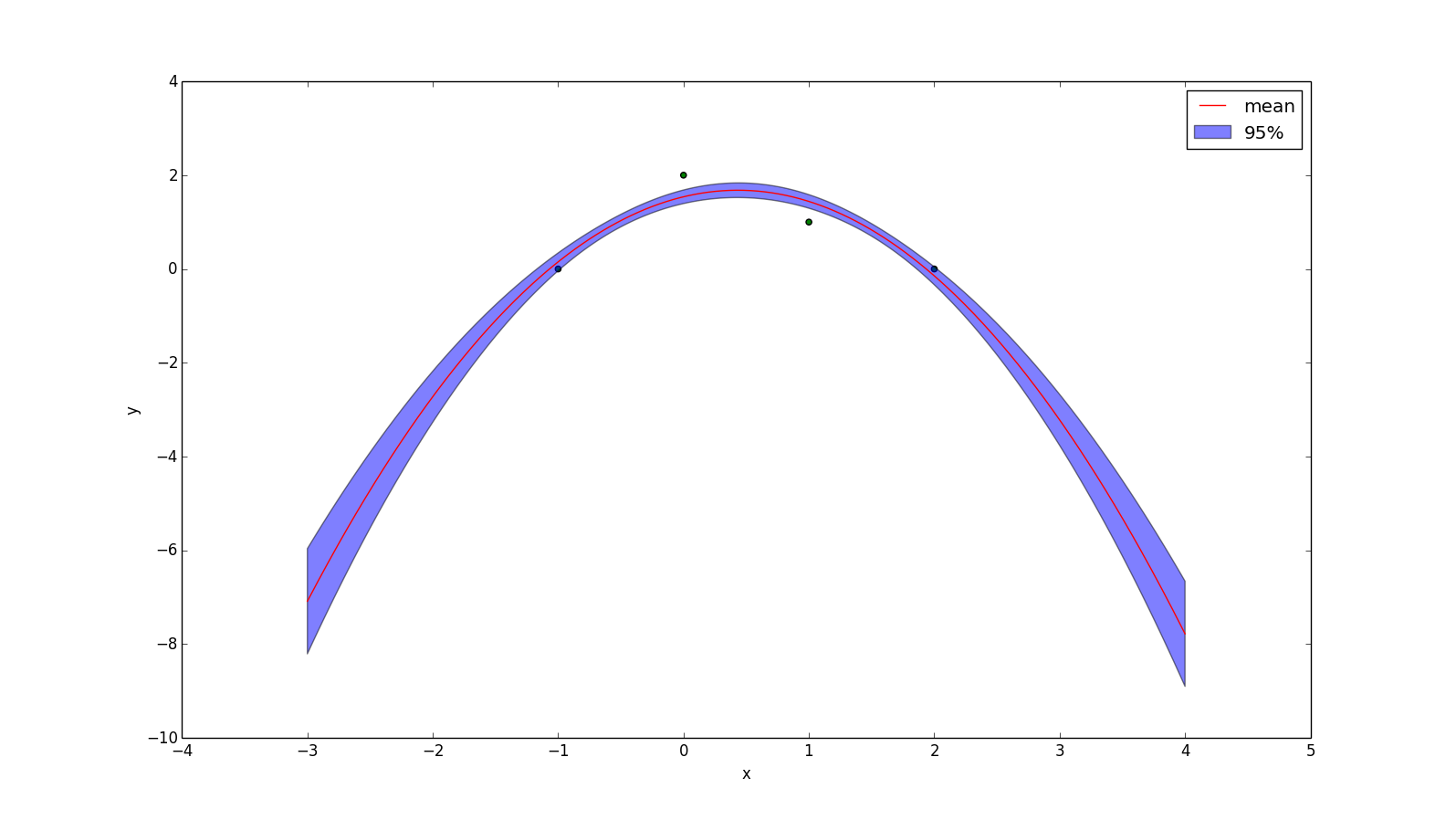
When $p=1$ the resulting mean function will be the least-squares regression line. When $p=2$ it will be the least-squares quadratic curve. The plot below uses $p=2$ and a noise with standard deviation 0.1.
(Food for thought: if I don't add noise to this, the plotting program crashes. Why do you think that is?)
-
An unpopular kernel is the Dirac delta function:
\[k(x_1, x_2) = \delta(x_1 - x_2)\]
But for didatic purposes, here is the plot:
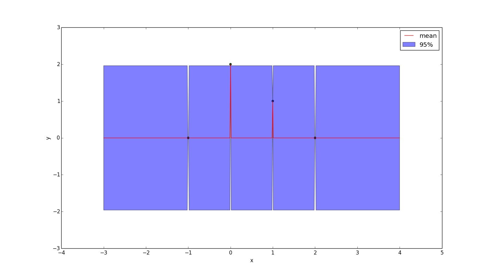 This kernel assumes there is no relationship between points!