Principle Component Analysis

Overview

If you have a high-dimensional dataset, it's often useful to see if you can remove a few dimensions without significant loss of information. For instance, you might want to collapse people's answers to hundreds of personality questions down to 5 personality traits, or people's answers to hundreds of political questions down to 2 political axes.

You can also take two dimensions down to one:

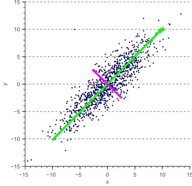
As you can see just by looking at the "cloud" of points, the green vector captures the vast majority the variance in points. We're going to discuss how PCA can help us find these high-information directions.

Theory

Imagine you had $n$ points with dimension $m$. We're going to represent this dataset as an $n \times m$ matrix $X$ with rows corresponding to points and columns corresponding to dimensions. In particular, we will denote dimension $j$ of point $i$ as $X_{ij}$. We're going to assume our data is centered at 0 to simplify the calculations.

Recall that given two vectors, $\vec{a}$ and $\vec{b}$, we can compute the projection of one onto the other using the dot product:

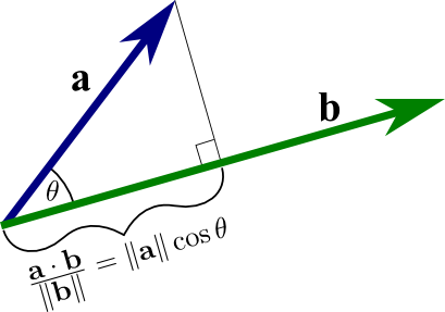
It turns out that if we interpret $a$ as a point in our dataset and $b$ as a vector, this projection is equal to the (signed) distance of $a$ along the $b$ direction, so if we square the dot product, we will will get how much variance point $a$ has along vecotr $b$. If we also require that $b$ be a unit-vector, then we can even drop the denominator and just say that the variance captured equals $(\vec{a} \cdot \vec{b})^2$.

So, we're trying to find a unit vector $\vec{u}$ that captures the most variance. Mathematically, we are trying to find $$\max_\vec{u}{\sum_i^n{(X_i \cdot \vec{u})^2}}$$

Some thought should convince you that that this is equivalent to saying $$\max_\vec{u}{\lvert X \vec{u} \rvert^2}$$ which is equivalent to $$\max_\vec{u}{\vec{u}^T X^T X \vec{u}}$$

Some math magic allows us to conclude that $\vec{u}$ must be the eigenvector of $X^T X$ with the largest eigenvalue.

Having thus found the vector that explains the most variance, we can repeat this process with the residuals to greedily explain the as much variance as possible.

This iterative process is equivalent to simply computing all the eigenvectors of $X^T X$ and sorting them by the size of their eigenvalues (NOTE: since the matrix is positive semidefinite, the eigenvalues are all real and non-negative, though).

def pca(X, normalize=False, epsilon=1e-7):
  # Subtract the mean of each column
  X = X - X.mean(0)
  # Optionally normalize variances to 1
  if normalize:
    X /= X.std(0) + epsilon
  # Compute the covariance matrix
  cov = np.dot(X.T, X) / X.shape[0]
  # Compute eigenvalues and vectors of the covariance
  # matrix.  'linalg.eigh' assumes the matrix is real and symmetric -- you can
  # use 'linagl.eig', but may get some negative/complex values due to numerical
  # precision errors.
  values, vectors = np.linalg.eigh(cov)
  # Sort by eigenvalues
  I = np.argsort(-values)
  values = values[I]
  vectors = vectors[:,I]
  return values, vectors