Lagrange Multipliers
The Problem
Imagine you're walking along a path on a mountain. You want to know what the highest point you reach is. Lagrange multipliers (LM) is a technique to find this maximum.
In particular, let the mountain be defined by $f(x,y)$, and let your path be defined as $g(x,y)=0$. For instance, you could define a circular path as $x^2+y^2-1=0$; or, you could define a parabolic path as $y-x^2=0$.
Contour Maps
To understand LM, it's helpful to understand contour maps. Contour maps are used in Earth sciences to illustrate the elevations in an area, but they are also often shown in weather forecasts to show how pressure and temperature differs between regions:
In the map above, for instance, you can see that temperatures generally get warmer (higher) as you move south, but that some areas buck this trend. More specifically, in the map above each "contour" corresponds to a 5˚ change in temperature. We can similarly define a contour map for functions in mathematics. For instance, the function $z=x^2+2y^2$ has a contour map that looks like
Like in the temperature map, every point on a particular contour has the same height ($z$-value). We can see that the contours are "denser" along the $y$ direction, which makes sense since $z$ varies twice as much along the $y$ direction as along the $x$ direction. Likewise, since $z$ varies faster as you go away from the origin, the contours get denser.
The Idea
The fundamental idea behind LM is that the local minimums and maximums along the constraint occur when the constraint is parallel to the contours.
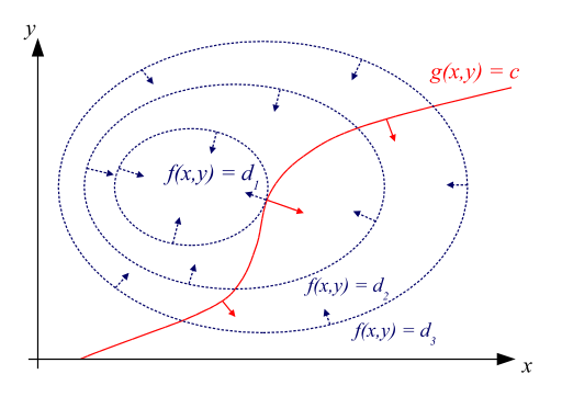
To understand why this is the case, imagine you were walking along $g$. When $g$ is moving parallel to the contours, your elevation isn't changing, which, you may recall from Calculus I, means you've reached a critical point. So now, we've reworded our problem of founding these "parallel points".
Recall, that $\nabla f$ returns the gradient of $f$, which means that $\nabla f$ will always point perpendicular to it's contour. This is represented by the blue arrows.
It turns out that $\nabla g$ yields a vector perpendicular to $g$ - though why this is the case is beyond the scope of this article. These perpendicular vectors are represented by the red arrows.
Therefore, we need to find points for which $\nabla f$ is parallel to $\nabla g$. This gives us the LM-method: find $\lambda$, $x$, $y$, and $z$ so that $$\nabla f(x,y,z) = \lambda \cdot \nabla g(x,y,z)$$
Example
Let's say you're trying to find the maximum value of $1-x^2-y^2$ along the line $y=2x+3$. Then, we can define $$f(x,y)=1-x^2-y^2$$ and $$g(x,y)=2x+3-y$$ So, our LM equation is $$ \left[ \begin{matrix} -2x \\ -2y \end{matrix} \right] = \lambda \cdot \left[ \begin{matrix} -2 \\ -1 \end{matrix} \right] $$
This gives us a system of 3 equations and 3 variables: $$ \begin{align} -2x &= -2\lambda \\ -2y &= -\lambda \\ 2x+3-y &= 0 \end{align} $$ Solving this yields $x=-2,y=-1,\lambda=-2$. If we plug this back into $f$, we get the extrema $(-2,-1,-4)$.
Multiple Constraints
LM can be extended rather intuitively if you have multiple constraints. Given constraints $g$ and $h$, the equation just becomes $$\nabla f(x,y,z) = \lambda \cdot \nabla g(x,y,z) + \mu \cdot \nabla h(x,y,z)$$