Income Tax Elasticity Literature
[ This page is my attempt at an unbiased review of the labor-tax elasticity estimation literature, much as one would get at a university. It is largely based on videos of lectures from Harvard, the cited papers, other reading. It is mostly based on this series of lectures Topic 5: Income Taxation and Labor Supply part 1. ]
The Model
Suppose each person has utility function
$$ u(c, L) = c - a \frac{L^{1+1/\epsilon}}{1+1/\epsilon} $$and non-labor income $y$ to yield consumption
$$ c = (1 - \tau) w L + y $$This implies
$$ \log(L) = \alpha + \epsilon \log((1-\tau)w) $$Often, an "income effect" variable is also added:
$$ \log(L) = \alpha + \epsilon \log((1-\tau)w) + \gamma y $$Note this entire model is "largely motivated by empirical tractability" (i.e. it's all a little bit bullshit).
One problem with this model is assumes people simply change the number of hours they work rather than choosing whether to work. This is sometimes modeled by adding an indicator variable using a logistic-esque model.
$$ \phi (\log(L) = \alpha + \epsilon \log((1-\tau)w)) $$Estimating $\epsilon$ From Kinks
[TODO: Go back to the kinks part. ]One way to estimate $\epsilon$ is to look at "kinks" in the tax system - that is, places where the marginal tax rate jumps. For instance, if the marginal tax rate jumps from $30% to 50% at $100k, we'd expect people's incomes to cluster just under $100k, with few people immediately over it. Obviously, estimates using the kink methodology runs into issues of inferring causation from correlation.
See the 58th minute of Topic 5: Income Taxation and Labor Supply part 1 for a discussion of "virtual incomes", which is basically equivalent to my insight where we can treat tax brackets as flat taxes with refunds. This is represented by the $y$ in our model. The video continues with a discussion of maximum likelihood estimation based on this insight.
The fundamental problem with this model is that it predicts significant bunching at these kinks. In reality, we see little bunching. In fact, a number of studies using this technique end up estimating negative elasticities.
Saez developed a second methodology for estimating elasticities from kinks, and while he also doesn't find much bunching for most people, but he does find significant bunching among the self-employed Do taxpayers bunch at kink points?, which most researchers think is due to *ahem* "income manipulation" rather than labor responses.
Other studies also look at social security recipients and estimate relatively large elasticities Friedberg Haider.
In general, though, there is very little kinking. Why? There are a few explanations:
- $\epsilon$ is, in fact, quite small.
- People can't perfectly predict their incomes, so they can't realistically target the kink. However, even though this is true, rational agents should still cause significant bunching behavior, which we don't see.
- People are "confused" by non-linear tax schedules. For instance, we know this is true regarding non-linear utility bills Ito.
Regarding the last point, recent research has found the amount of EITC bunching varies dramatically across zip-codes and there is some evidence this variation is due to variance in knowledge. As an aside, this study found that 73% of this bunching is from people working more and 27% from people working less.
Estimating $\epsilon$ from (Quasi) Experiments
The primary way economists estimate $\epsilon$ is by using tax reforms as natural experiments. There are some issues with this:
- It's difficult to measure hours worked, so economists frequently take income as a proxy, under the assumption that wages don't change much.
- Temporary tax changes cause larger labor changes than permanent ones, because people decided to work more hours while taxes are low to enable them to work fewer while taxes are high.
- The above model implicitly assumes a flat tax by using $\tau$ to represent both the marginal and effective tax rate. There are ways to deal with this that we'll get to later.
- Labor can take time to respond to tax changes. For instance, the way most people adjust their labor is by switching jobs.
Negative Income Tax Experiments
Famously, researchers have used negative income tax experiments to estimate $\epsilon$. For instance, in one study Ashenfelter, they varied (1) the transfer given to no-income people and (2) the phase-out rate. By comparing people with equal base transfers but different phase-out rates, we can estimate $\epsilon$. They generally found $\epsilon \approx 0.1$ for males and $\epsilon \approx 0.5$ for females. Unfortunately, this study used voluntary income reports and had high attrition rates in some groups, so it's hardly a gold standard.
In any case, most modern studies don't use these true experiments anymore, using instead quasi "natural" experiments.
Differences During Tax/Welfare Reforms
As an example, one research looked at the effect of the Tax Reform Act of 1986 on the labor decisions of married women Eissa. As most researchers do, she used a "differences of differences" approach, which I'll explain now.
Basically, the tax reform caused the marginal tax rates of married women to increase, but they increased more for the highest earning women:
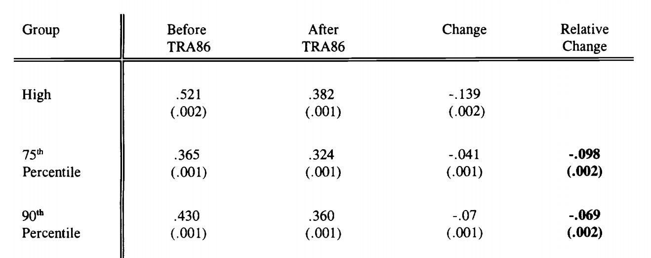
Consequently, the highest earning women reduced their labor by more:
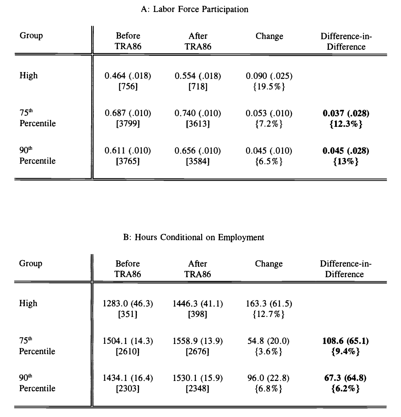
To estimate $\epsilon$ we simply divide these differences-of-differences. In this case, she estimates that $\epsilon \approx 0.4$ for labor force participation and $\epsilon \approx 0.6$ for hours worked, for a total elasticity of about 1, which is very high since it suggests we're on the top of the Laffer curve.
On the other hand, future work suggests this estimation method is biased upwards by the interaction of two facts: (1) elasticities are unequal across income levels and (2) even the low-income groups typically get some treatment. The math showing this bias is fairly straightforward arithmetic.
Another significant issue is that tax reforms cause people to take actions to reclassify their income to minimize their tax burden. This also makes elasticity estimates biased upwards.
Finally, top earners also have some ability to determine when to realize their incomes from year to year. We can account for this by choosing pre-announced tax reforms and changing our regression from
$$ \alpha + \beta \log(1-\tau)$$to
$$ \alpha + \beta_1 \log(1-\tau_t) + \beta_2 \log(1-\tau_{t+1})$$and then estimating the long-run elasticity as $\beta_1 + \beta_2$. Applying this methodology to the effects of the Clinton tax cuts on top executives changes the $\epsilon$ estimate from ~1.2 to ~0.4 Goolsbee. Using more adjustments makes the estimate even smaller.
This diff-in-diff methodology is more difficult to do to non-top-earners, because you have to adjust for the fact that the tax change can change people's brackets, not just their rates.
TODO: Continue @ 21:00 from here.
...
One popular topic of research has been the effects of the mid-90s welfare reforms. These reforms are ideal of statistical analysis since they include a quasi experiment that differs across time and across states, since states had considerable autonomy in these reforms.
The research has generally found that the reforms increased the labor supply with minimal negative effects on consumption. However, there is skepticism that these conclusions are broadly applicable given the booming economy of the 90s.
Grouping Instruments
Another attempt partitions the wage data into cells (e.g. year, age, gender, and education) and then computes the mean wage of each cell Blau. [ TODO: figure out how this grouping instruments works from 25:00 from "Topic 5: Income Taxation and Labor Supply part 3". ]
They end up concluding that $\epsilon$ shrank from ~0.4 in 1980 to ~0.2 today, approaching the low elasticities of men.
Other Bits
Estimating $\gamma$
A study from lotteries estimates that for every dollar they gain in non-labor income, most people reduce their labor income by ~10¢ Imbens.
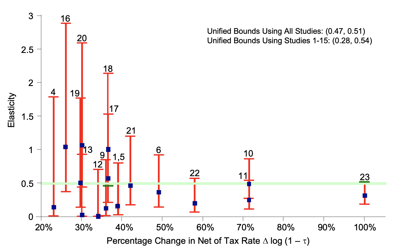
Frictions
Chetty proposes that people only actually shift their labor if the tax change causes a large enough gap between current and optimal utility. If we assume people only change their $L$ when this gap is larger than some amount ($\delta$), we must conclude that our estimates of $\epsilon$ have significant additional error Bounds on elasticities with optimization frictions. For instance, if we assume $\delta$ is 1% of income, then we find we ccan make all the studies agree:
A literature review using this friction model estimates that the intensive $\epsilon \approx 0.33$ and $\epsilon \approx 0.21$ Are micro and macro labor supply elasticities consistent? A review of evidence on the intensive and extensive margins.